Localize a mobile robot in a virtual environment with constraint programming.
In the last post, I presented quickly constraint programming, with a lot of text and a single real example. In this one I will show a SLAM (Simultaneous Localization And Mapping), able to localize a mobile robot in an unknown virtual environment.
Here, we consider that the robot position at t0 is known, as well as it’s sensors information (velocity and orientation). During his journey in the virtual world, our robot will use simulated LIDAR data which will allow him to detect distance and orientation of this world’s markers (with an unknown position). We also consider that we know which marker as been spotted.
All those measures obviously have a margin of error that we know (in the real world, this information are obtained with the sensor documentation). However, our small virtual world cannot have outliers in the measured data.
This system cannot work in the real world of real life.
For this project, I used Tubex, a constraint programming library for C++ and Python, allowing us to use tools to work on constraint trajectories. My implementation is an improvement of the last tutorial example (Range Only SLAM).
To estimate the performances of our SLAM, we will define an initial point of comparison : the trajectory estimation with dead reckoning. Dead reckoning estimates the position with a direct sensor integration of the sensors values, a bit like estimating your position after closing your eyes and just counting your steps as someone walks you somewhere. It’s a simple solution to robot positioning problems, but it accumulates quickly errors.
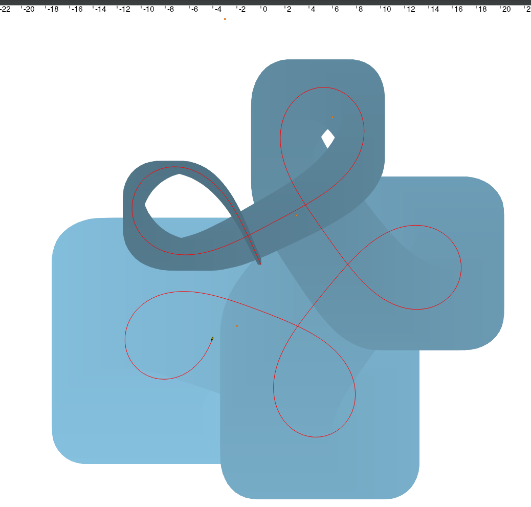
Tubex represents uncertainty on trajectories by using tubes, displayed with a gradient of color.

On the image I displayed the dead reckoning trajectory of the robot in blue, and the real trajectory in red. The uncertainty of the robot position grows with time, hence the widening of the blue trajectory, until we reach the final position, with an uncertainty interval of 18x18 meters. It’s starting point is the point with the less uncertainty, where the blue trajectory is narrow. Contraint programming allows us to get the final dead reckoning trajectory including all the possible positions of our robot, even with a low precision (the red trajectory never goes out of the blue one).
The four markers on the map are displayed as orange squares, and their position are unknown to the robot.
This trajectory is our starting variable, which will be constraint by our program as the map becomes known.
A V1
Lets jump right into it and see the result:

Well what can we see on this image ? The gray part is the dead reckoning trajectory, which was reduced to the blue part. We can notice right away that the estimated position for the robot is much better than before: we are in a final interval of 2x1 meter, an improvement of 99.38%.
We can also see rectangles around the markers, which are the interval of the estimated positions of each marker at the end of the mapping process. As for the robot, their final positions are in an interval.
A V2 !
Well, the result of V1 is good and all, but a bit useless: our robot is already at its destination when we estimate its position through time. A more useful information would be to obtain the robot position at each t, and that’s what I’ll do now.
Our code does not need a lot of modification: we only need to obtain the position (and reduce the variables) more regularly than just once at the end.

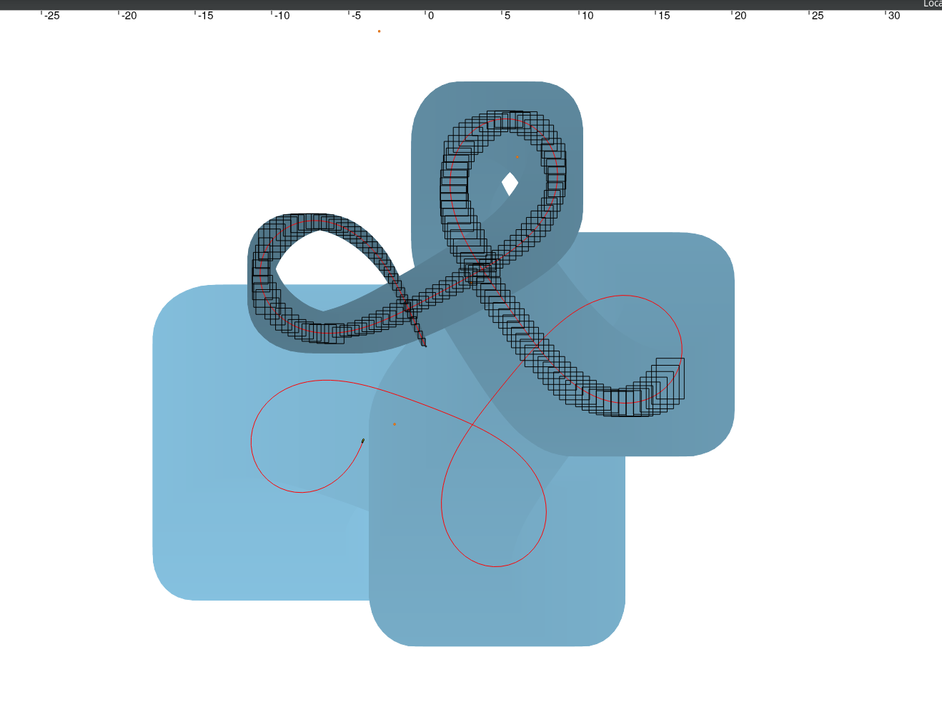
This time the dead reckoning trajectory is not contracted, and is just displayed as a comparison. The robot position at each t is displayed as a black interval.
The instantaneous position estimation will be of lower quality than V1, because we can’t have access to all the data for each position estimation. But once we got to the end, the final trajectory is contracted one last time be taking all data into account, and we obtain the exact same trajectory as V1.