After tackling the procedural generation of planetary systems, I decided to step up a bit in universe and try to take on galaxies
Here, we want to keep some conditions in mind. Those conditions are basics for an observer, placed anywhere in the galaxy:
- Most shinny stars are visible from afar
- Close stars can be seen even with a low brightness
- The galactic model must be defined for every point (x, y, z)
Define the shape
When we say “Galaxy”, we usually think about a sort of planar spiral structure with a bulge in the center.
In our universe, we can see various (an infinity of) other shapes, from spirals to sombrero, from barred spirals to shapeless (irregular galaxies). Here, we only care about spiral galaxy generation, in my opinion the nicest and those with the most difficult shape to define with an algorithm.
For the spiral shape, I decided to go with A New Formula Describing the Scaffold Structure of Spiral Galaxies, describing a formula easy enough to parametrize, and with a good approximation of what we can find in nature. It is based on a log spiral, with variations allowing to link naturally the arms to the central bar.
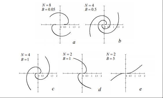
It defines the shape of a spiral galaxy in polar coordinates with the following equation: $$ r(\phi) = \frac{A}{ log(B \tan\frac{\phi}{2N}) } $$ With A a scale parameter, B and N to control the degree and slope of the spiral.
Some exemples with A = 1:
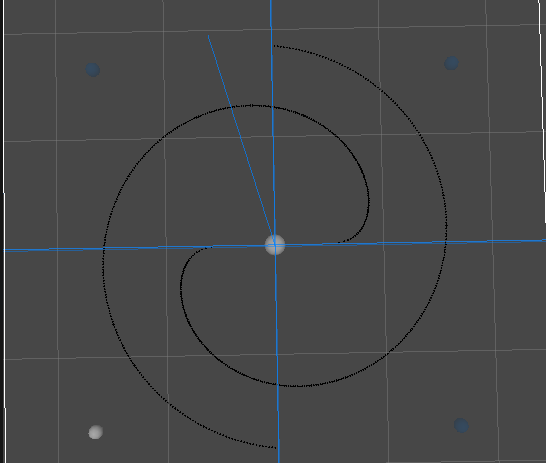
I implemented this equation in a way allowing me to use it as a density function of space : We take a point (x, y, z) in space and the function returns the star density of our galaxy at this point.
Here is a little two armed galaxy:
Define densities
Once the shape defined, I laid out a general algorithm to obtain the density at each point depending on where we are:
Bulge
The heart of our galaxy is a simple inverse exponential equation. I decided to use de Vancouleurs law.
$$ d_{bulge}(r) = I_0 e^{-K r^{0.25} - 1} $$
With r the normalized distance to the center of the galaxy (between 0 and 1), K a parameter changing the diminution of density with distance (> 0), I0 a multiplier for the final value.
Global Density
The arms are also modelled with an inverse exponential : $$ d_{arms}(r) = I_0 e^{-K Br^{0.25} - 1} * e^{-\frac{r - Br}{R_5} } $$
With Br the normalized radius of the central bulge (between 0 & 1), and R5 the distance at which the density passes below 0.5.
This formula is used with a similar equation as the first one, to control the diminution of density when we get further from the center of the arm.
We switch from equation 1 to equation 2 in with our distance from the center:
    if (r < Br)
        //use bulge density
    else
        //use arms density
Result of the law of density for the parameters I0 = 2, Br = 0.1, K = 0.2, R5 = 0.2, function of the normalized radius:
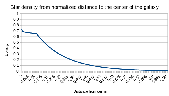
This equation can describe the density of stars in a galaxy of any shape, and we must add a density formula for the arms.
Arms
$$ d_{from arms} = e^{-\frac{Da}{Ra}}. $$
With Da the distance from the closest arm and Ra the normalized arm radius.
And here is our arms, with 4000 stars.
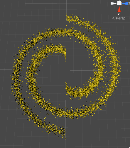
We can observe that density is higher when we get closer to the center of the galaxy, and center of the arms (Bulge and arm not displayed).
400 billion stars without burning RAM
In our dear Milky Way, we have an estimate of around 200 to 400 billion stars. Stars from Earth are visible (with a naked eye) because they emit light, and they are close to us. In fact, we can expect that very bright stars are visible from afar, and close stars can also be seen even if they emit dimly.
However, the brightest stars are also the rarest (B and O class), while the most numerous and also closest from Earth are very dim in comparison (M and K class). To avoid generating in memory the billion of stars in our galaxy and make my computer explode, it would be wiser to generate only the visible stars from our observing point.
Inspired by the Journal de Ysaneya, I decided to use an octree (briefly explained, the 3D struct of a 2D binary tree), splitting my galaxy in 8 principal cubes, which can also be divided in 8, and on and on until we reach a certain scale. The biggest cubes are placed at “level 0”, until the smaller ones at “level 12”.
The observer is in a cube of level 12, that mean in a cube taking 1/4096 of the all galaxy. For the Milky Way, it should represent a cube 126.9 x 126.9 x 126.9 light years, enough to contain the Sun and it’s close neighbors, and that represent already a big amount of stars (take a look at the Sun neighborhood at 250 LY).
An ilage of the subdivided octree to level 12, with a few stars generated with uniform density.
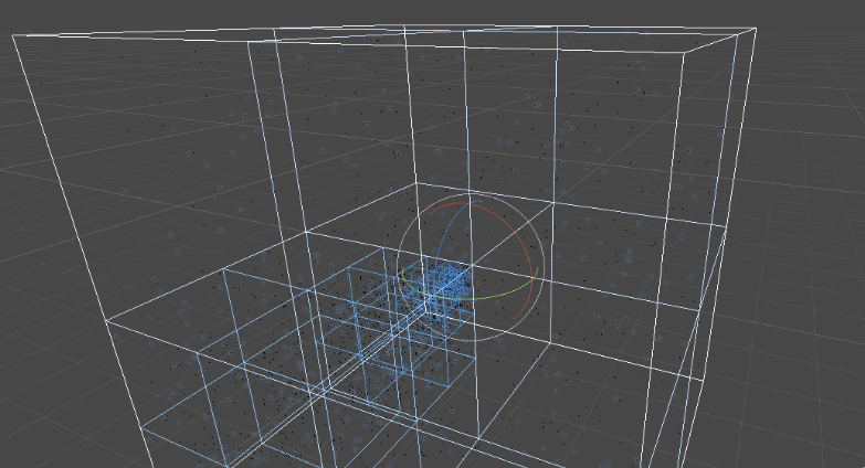 We can see that even with a uniform density, the stars are much more present around the observer.
Each level of the octree posses a spawning probability of star: the lower levels (0-3) favor the very bright stars, visible from afar, but rare in our galaxy (<1-2% of all stars). Intermediate level (4-9) are used for stars dimmer than O and B, but also much more frequent. The following levels are handling the very dim stars, which are also the most numerous, like yellow, orange and red dwarfs. The last level can also handle the special stars, like white dwarfs, failed stars (K, J, …) and maybe black holes.
In conclusion, using the structure of the octree, we guarantee that the far bright stars will be generated as well as the close dim stars, without generating all stars.
I did not yet think about a reliable solution to handle black hole and nebulas. I also currently search for a method to make the octree stars probabilities much more procedural than entering them by hand, to obtain more diverse and interesting results.